Problem statement
The cost of acquiring enough high-fidelity (HF) data from heavy simulations or experiments can be daunting. When much cheaper but less accurate low-fidelity (LF) data is available, multi-fidelity modeling 1 methods augment the limited HF data with cheaply-obtained LF approximations.
The Bayesian paradigm provides a coherent approach for specifying sophisticated hierarchical models: The HF data (evidence) update the posterior (our target) model conditioned on the prior model (belief) that is constructed from LF data. In this post, I demonstrate Bi-fidelity modeling performance on a toy model using a Bayesian Neural-Network ensemble and compare it with the Gaussian Process.
In addition, the Bayesian paradigm propagates uncertainties between fidelities. This is very useful information for surrogate-model-based decision-making. A notebook of this work can be found here
1. Toy Model
Let the toy model be in the following form:
\[y = A x^2 - B \exp{ \left(\sum_i^n c_i \cos (w_i x-b_i)\right)}\]where the parameters are arbitrarily chosen such that the HF and LF are slightly different as shown below:
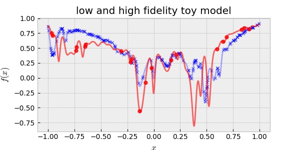
Throughout this post, we consider a scenario that the cost of LF data acquisition is less than one-tenth of the cost of the HF data acquisition. For example, the cost of acquiring 40 high-fidelity data is more expensive than the cost of acquiring 20 high-fidelity data and 200 low-fidelity data. In this regard, the data shown in the plot are randomly chosen 200 points for LF and 20 for HF. Note that all the data points are noiseless, i.e., they are well aligned with the ground truth toy model. Therefore, we expect that a good surrogate model to well capture the model uncertainty (epistemic uncertainty) not the data uncertainty (i.e., risk or aleatoric uncertainty).
2. Gaussian Process (GP)
2.1 Single Fidelity GP
Here, single fidelity GP is trained on the HF data. To be fair, I used 40 HF data ( which is more expensive than 20 HF data and 200 LF data by assumption ) to train GP. The RBF kernel is assumed and its hyperparameters are optimized for maximum likelihood of data. The following plot shows the result.
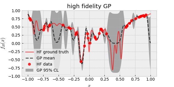
Observe that where the data points are few, GP predicts large uncertainty (. Note also that the HF ground truth is well within the GP predicted uncertainty.
2.2 Linear bi-fidelity GP
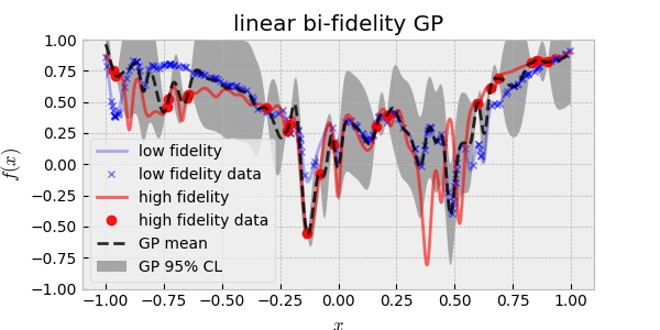
One of the widely used methods of multi-fidelity modeling is to assume that the HF and LF functions are related linearly:
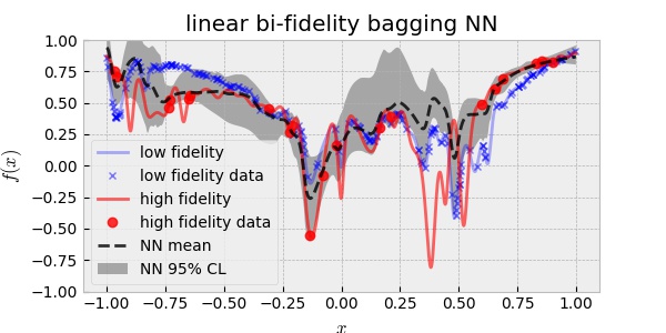
\[f_H(x) = f_{\text{err}}(x) + \rho \,f_L(x)\]where $f_{\text{err}}(x)$ and $f_L(x)$ are assumed to be independent GP and $\rho$ is a scalar scaling factor. This can be a good approach when $f_H(x)$ depends linearly on $f_L(x)$. Using 20 HF and 200 LF data, the linear bi-fidelity GP resulted in:
2.3 Nonlinear bi-fidelity GP
The linear approach, however, will fail when $f_H(x)$ and $f_L(x)$ are nonlinearly related. In this case, the nonlinear multi-fidelity GP assumes the following:
\[f_H(x) = f_{\text{err}}(x) + \rho (\,f_L(x) )\]This approach is called deep GP in analogous with deep neural network. Again, using 20 HF and 200 LF data, the nonlinear bi-fidelity GP resulted in:
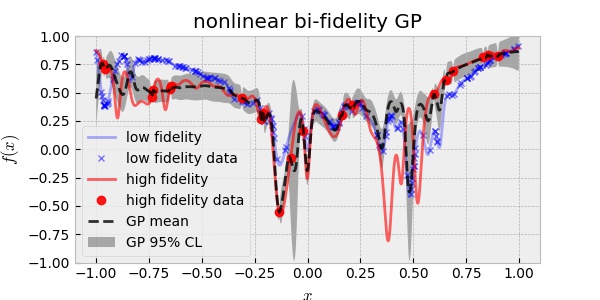
Although the nonlinear assumption between the two fidelities is more general than the linear assumption, the result above is disappointing in the sense that it is over-confident. In other words, the uncertainty prediction did not cover the true HF curve. This may be ascribed to the fact that the two fidelities of our toy model are very close to each other more linearly than nonlinearly.
3. Bootstrap aggregating (Bagging) Neural-Networks (NN)
Although GP is an exact Bayesian method, the computational complexity renders it impractical (without approximation) for high-dimensional problems. Here, we use the ensemble neural network method to construct the bi-fidelity bayesian surrogate model. The principle of ensembling for uncertainty quantification is:
- Each NN tends to converge where the data points are close by. However, they can vary from each other over the regions (of input domain) where data is absent.
Specifically, I use Bagging2 of NNs. Using different bootstrapped data to train each NN can further help to avoid overfitting.
3.1 Single fidelity Bagging NN
For performance comparison against the bi-fidelity model, here, we used 40 HF data to train Bagging NNs
Note that the truth in $x\in(0.25,0.75)$ is far from the mean of the prediction but also it is not within the prediction of the uncertainty. The bias of the mean can be understood by the lack of data. However, the overconfident uncertainty prediction is problematic (compare it with the single fidelity GP case): It suggests that Bagging NNs are not enough. We will cover this topic in other posts.
3.2 Bi-fidelity Bagging NN
In order to build the bi-fidelity model in a Bayesian way, I first created the prior belief: The ensemble NNs trained using bootstrapped data out of the 200 LF data. Then each the LF NN model is connected to the output of a new NN which represent the HF model that is going to be trained using HF data. Specifically, I represent the linear relation b/w the LF and HF model
\[f_H(x) = f_{\text{err}}(x) + \rho \,f_L(x)\]using the following structure.
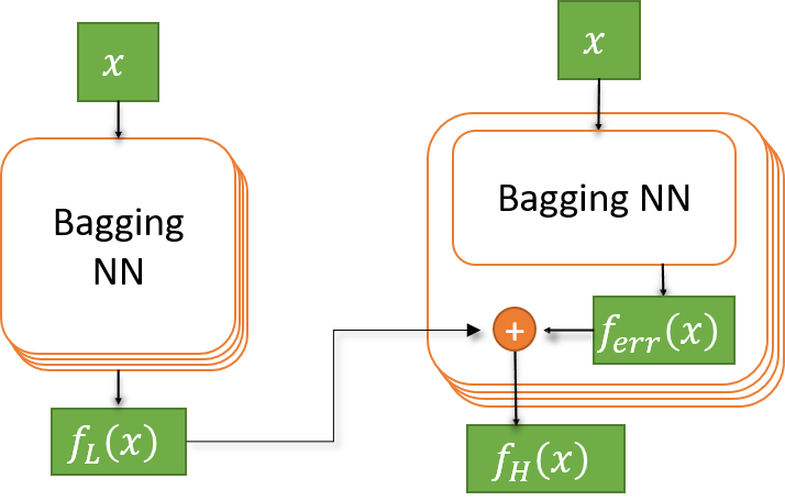
Note that this way, the NNs on the right predict the HF target function conditional to the LF surrogate model. By ensembling them, we are constructing the prior probability from LF Bagging NNs and the conditional probability from HF Bagging NNs
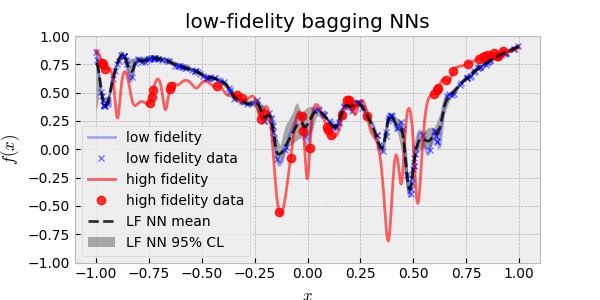
The following is the plot of the LF surrogate model trained using 200 LF data.
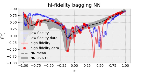
Once, I built the prior, I used the 20 HF data to train the HF surrogate model. The following plot is the result.
Observe that the prediction is better than the single fidelity result. Again, the bias of the mean in $x\in(0.25,0.75)$ can be understood by the lack of HF data. And again, the uncertainty prediction does not cover the ground truth of the HF target function. This result suggests again that Bagging NNs are not enough for uncertainty quantification for this problem. We will cover this topic in other posts.
4. Conclusion
I constructed the bi-fidelity model using Bagging NNs in a Bayesian way and compared it with the bi-fidelity gaussian process. I experimented with them on a regression problem over a toy model and observed that the bi-fidelity model prediction outperform the single fidelity model. I also find that the naive application of Bagging NN is not enough for epistemic uncertainty quantification in this toy model where the target function has high-frequency content. I suspect that the problem is due to the frequency bias of NN. I will cover this problem in a separate post.
Thank you, please contact me to leave any comments or questions email Github discussion
References
1. Multifidelity Modelling, https://mlatcl.github.io/mlphysical/lectures/05-02-multifidelity.html
2. Bagging,https://www.stat.berkeley.edu/~breiman/bagging.pdf
3. Dropout as a Bayesian Approximation: Representing Model Uncertainty in Deep Learning, https://arxiv.org/pdf/1506.02142.pdf
4. Risk versus Uncertainty in Deep Learning: Bayes, Bootstrap and the Dangers of Dropout, http://bayesiandeeplearning.org/2016/papers/BDL_4.pdf